Project Overview
While the Borderland’s franchise is renowned for its unprecedented number of weapon combinations, the existing "score" metric and lack of playstyle classifier offers lackluster insight into weapon quality, often falling short for players seeking a deeper understanding of their gear for their preferable playstyle, therefore, highlighting the need for a more precise and comprehensive metric. This project aims to address these gaps by developing a data-driven metric and using machine learning techniques to classify gun types further suitable for a player’s playstyle. By incorporating advanced visualization tools such as autoencoders and PCA, we aim to reveal hidden relationships between attributes like gun type, rarity, and our new metric, thereby improving player gear comprehension and engagement.
Data Gathering and Cleaning
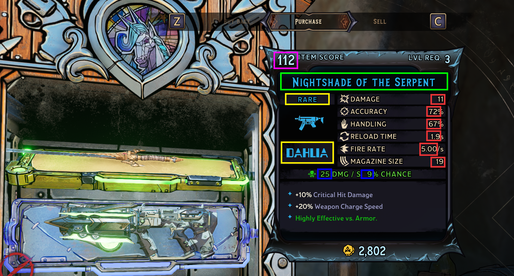
The data had to be extracted directly from the source which meant using Machine Learning OCR (Optical Character Recognition) techniques to digitize and extract data from screenshots of the game. After extraction, extensive cleaning and validation processes were performed to ensure data accuracy, workability, and consistency.
import pyautogui
import time
import cv2
import pytesseract
import pandas as pd
import numpy as np
import easyocr

reader = easyocr.Reader(['en'], gpu=False)
pytesseract.pytesseract.tesseract_cmd = r'C:\Program Files\Tesseract-OCR\tesseract.exe'
time.sleep(10)
weapon_data = []

def capture_screen(region):
    #screeshot the region for ocr
    screenshot = pyautogui.screenshot(region=region)
    screenshot = cv2.cvtColor(np.array(screenshot), cv2.COLOR_RGB2BGR)
    return screenshot

def extract_text(image):
    #use easyocr to extract text
    result = reader.readtext(image, detail=0)
    return ' '.join(result).strip()

def extract_numeric_text(image):
    #restrict OCR to recognize only numbers, periods, and commas
    config = '--psm 6 -c tessedit_char_whitelist=0123456789.,'
    text = pytesseract.image_to_string(image, config=config)
    return text.strip()


def calculate_region_coordinates(tlx, tly, brx, bry):
    width = brx - tlx
    height = bry - tly
    return (tlx, tly, width, height)
import cv2

def preprocess_image(image, thresholding=True, resize=True, scale_factor=2):
    #grayscale
    gray = cv2.cvtColor(image, cv2.COLOR_BGR2GRAY)

    #thresholding
    if thresholding:
        _, gray = cv2.threshold(gray, 150, 255, cv2.THRESH_BINARY)

    #upscale image
    if resize:
        gray = cv2.resize(gray, None, fx=scale_factor, fy=scale_factor, interpolation=cv2.INTER_CUBIC)
    return gray

def shotgun_check(image):
    #checks if the image is a shotgun
    if extract_numeric_text(image) == '80':
        return True
    return False

# screen regions on my 2560x1440 monitor
WEAPON_NAME_REGION = calculate_region_coordinates(1181, 245, 1747, 307)
WEAPON_STATS_REGION = calculate_region_coordinates(1598,310,1735,556)

WEAPON_DAMAGE_REGION = calculate_region_coordinates(1610,311,1735,348)
WEAPON_ACCURACY_REGION = calculate_region_coordinates(1610,352,1735,390)
WEAPON_HANDLING_REGION = calculate_region_coordinates(1610,396,1735,430)
WEAPON_RELOAD_SPEED_REGION = calculate_region_coordinates(1610,435,1735,473)
WEAPON_FIRE_RATE_REGION = calculate_region_coordinates(1610,480,1735,515)
WEAPON_MAGAZINE_SIZE_REGION = calculate_region_coordinates(1610,521,1735,555)

WEAPON_RARITY_REGION = calculate_region_coordinates(1187,313,1364,347)
WEAPON_MANUFACTURER_REGION = calculate_region_coordinates(1189,473,1365,547)
WEAPON_TYPE_REGION = calculate_region_coordinates(1521,1228,1577,1257)
WEAPON_ITEM_SCORE_REGION = calculate_region_coordinates(1164,177,1240,220)
WEAPON_ELEMENTAL_DMG_REGION = calculate_region_coordinates(1300,561,1346,594)
WEAPON_ELEMENTAL_CHANCE_REGION = calculate_region_coordinates(1450, 561, 1520, 596)

#automation
def refresh_and_collect():
    pyautogui.press(']')  #vending refresh key
    time.sleep(1)  #wait for refresh
    pyautogui.press('e')  #open shop
    time.sleep(0.5)

    #scrolling shop
    for item in range(10):  #num of items in shop
        #get name and stats
        name_img = capture_screen(WEAPON_NAME_REGION)
        rarity_img = capture_screen(WEAPON_RARITY_REGION)
        manufacturer_img = capture_screen(WEAPON_MANUFACTURER_REGION)
        damage_img = capture_screen(WEAPON_DAMAGE_REGION)
        accuracy_img = capture_screen(WEAPON_ACCURACY_REGION)
        handling_img = capture_screen(WEAPON_HANDLING_REGION)
        reload_speed_img = capture_screen(WEAPON_RELOAD_SPEED_REGION)
        fire_rate_img = capture_screen(WEAPON_FIRE_RATE_REGION)
        magazine_size_img = capture_screen(WEAPON_MAGAZINE_SIZE_REGION)
        item_score_img = capture_screen(WEAPON_ITEM_SCORE_REGION)
        type_img = capture_screen(WEAPON_TYPE_REGION)
        elemental_dmg_img = capture_screen(WEAPON_ELEMENTAL_DMG_REGION)
        elemental_chance_img = capture_screen(WEAPON_ELEMENTAL_CHANCE_REGION)

        item_score = extract_numeric_text(item_score_img)
        rarity = extract_text(rarity_img)
        name = extract_text(name_img)
        if shotgun_check(type_img):
            damage = extract_text(damage_img)
        else:
            damage = extract_numeric_text(damage_img)
        Edamage = extract_numeric_text(elemental_dmg_img)
        Echance = extract_numeric_text(elemental_chance_img)
        accuracy = extract_numeric_text(accuracy_img)
        handling = extract_numeric_text(handling_img)
        reload_speed = extract_text(reload_speed_img)[:-1]
        fire_rate = extract_numeric_text(fire_rate_img)
        magazine_size = extract_numeric_text(magazine_size_img)
        manufacturer = extract_text(manufacturer_img)

        name = name.replace('\n', '')
        damage = damage.replace('\n', '')
        accuracy = accuracy.replace('\n', '')
        handling = handling.replace('\n', '')
        reload_speed = reload_speed.replace('\n', '')
        fire_rate = fire_rate.replace('\n', '')
        magazine_size = magazine_size.replace('\n', '')
        Edamage = Edamage.replace('\n', '')
        Echance = Echance.replace('\n', '')
        rarity = rarity.replace('\n', '')
        manufacturer = manufacturer.replace('\n', '')
        #if manufacturer contains SWIFT or KLEAVE skip appending since those are melee weapons
        if 'SWIFFT' in manufacturer or 'KLEAVE' in manufacturer:
            pyautogui.press('s')
            time.sleep(0.1)  #wait for scroll
        else:
            weapon_data.append([item_score, rarity, name, damage, Edamage,
            Echance, accuracy, handling, reload_speed, fire_rate, magazine_size, manufacturer])
            pyautogui.press('s')
            time.sleep(0.1)  #wait for scroll
    pyautogui.press('esc')  #exit vending machine

#loop change range for more or less weapon data collection
for loop in range(800): #num of loops
    refresh_and_collect()
    print(f"Loop {loop+1} completed.")

#export data
df = pd.DataFrame(weapon_data)
df.to_csv('weapon_data.csv', index=False)
Key Design Features:
- Using Screen Coordinates for Screenshots: Allowed for collection of data without intrusive methods on the game
- Machine Learning OCR: Converted the screenshots into numerical data so I could perform analysis on it
- Data Structuring: Sturctured and Exported the extracted data in a csv format to enhance future readabiliy and usability
Here is the code for the preprocessing of the extracted code, it orginally was written in a python notebook which is why the # %% symbols are present. Each of the symbols represents a different code block which I used to separate my processing so I can ensure accurate data validation.
# %%
import pandas as pd
import numpy as np
import seaborn as sns
import matplotlib.pyplot as plt
# %%
# importing data from the extraction code
data_nomf = pd.read_csv('weapon_data2.csv')
data1000 = pd.read_csv('weapon_data3.csv')
data4000 = pd.read_csv('weapon_data5.csv')
data4000.head()
# %%
#add string column for manufacturer to data_nomf
data_nomf['manufacturer'] = data_nomf['2'].str.split().str[0]
# %%
#rename columns for all three dataframes
data_nomf.columns = ['item score', 'rarity', 'name', 'damage', 'elemental damage',
'elemental chance', 'accuracy', 'handling','reload speed','fire rate','magazine size','manufacturer']
data1000.columns = ['item score', 'rarity', 'name', 'damage', 'elemental damage',
'elemental chance', 'accuracy', 'handling','reload speed','fire rate','magazine size','manufacturer']
data4000.columns = ['item score', 'rarity', 'name', 'damage', 'elemental damage',
'elemental chance', 'accuracy', 'handling','reload speed','fire rate','magazine size','manufacturer']
#combine dataframes
data = pd.concat([data_nomf, data1000, data4000])
data.head()
# %%
len(data)
# %%
#capitalize the entire name column
data['name'] = data['name'].str.upper()
data.head()
# %%
#possible gun names and their manufacturers
guns_by_manufacturer = {
"DAHLIA": [
"MALLORN", "TAMARACK", "THUMBSBANE", "BARB", "THORN",
"NIGHTSHADE", "FOXGLOVE", "HEMLOCK", "GREENSPINE",
"NETTLE", "MAGNOLIA", "BANYAN"
],
"BLACKPOWDER": [
"TINTACK", "BOILERMAKER", "STOVEPIPE", "HOBNAIL",
"RIVETER", "RATCHET", "RAILSPIKE", "PUSHPIN",
"PINION", "HELICAL", "KETTLEDRUM"
],
"HYPERIUS": [
"BASILISK", "EIDOLON", "FAE", "KOBOLD",
"MANTICORE", "MYTHOPEIA", "PARABLE", "SAGA",
"SPRIGGAN", "WRAITH"
]
}
#extract first word from name column and save the rest of the name in a new column
data['gun name'] = data['name'].str.split().str[0]
data['rest of name'] = data['name'].str.split().str[1:].str.join(' ')
data['gun name'].unique()
# %%
#replace invalid gun names with their correct names
data['gun name'] = data['gun name'].replace('BOLLERMAKER','BOILERMAKER')
data['gun name'] = data['gun name'].replace('BOLERMAKER','BOILERMAKER')
data['gun name'] = data['gun name'].replace('BOJLERMAKER','BOILERMAKER')
data['gun name'] = data['gun name'].replace('EDOLON','EIDOLON')
data['gun name'] = data['gun name'].replace('HUMBSBANE','THUMBSBANE')
data['gun name'] = data['gun name'].replace('ELDOLON','EIDOLON')
data['gun name'].unique()
# %%
#change the manufacturer of the guns to the correct manufacturer based on the gun name
def find_manufacturer(gun_name, guns_dict):
for manufacturer, guns in guns_dict.items():
if gun_name in guns:
return manufacturer
return "No Match"
data['manufacturer'] = data['gun name'].apply(lambda x: find_manufacturer(x, guns_by_manufacturer))
#drop the gun name column
#data = data.drop(columns=['gun name'])
#delete the words OF and THE from the rest of name column
data['rest of name'] = data['rest of name'].str.replace('OF','')
data['rest of name'] = data['rest of name'].str.replace('THE','')
#move the gun name and rest of name columns to where the name column was
data = data[['item score', 'rarity', 'gun name', 'rest of name', 'damage', 'elemental damage',
'elemental chance', 'accuracy', 'handling','reload speed','fire rate','magazine size','manufacturer']]
data.head()
# %%
#remove damage rows where damage is nan
data = data.dropna(subset=['damage'])
len(data)
# %%
data['elemental damage'].unique()
# %%
#trim all periods from elemental damage
data['elemental damage'] = data['elemental damage'].str.replace('.', '')
data['elemental chance'] = data['elemental chance'].str.replace('.', '')
data['elemental damage'] = data['elemental damage'].str.replace(',', '')
data['elemental chance'] = data['elemental chance'].str.replace(',', '')
#drop rows where elemental damage is ''
data['elemental damage'] = data['elemental damage'].fillna('0')
data['elemental chance'] = data['elemental chance'].fillna('0')
data = data[data['elemental damage'] != '']
data['elemental damage'].unique()
# %%
#plot elemental damage for distribution
data['elemental damage'] = data['elemental damage'].astype(int)
sns.boxplot(data['elemental damage'], orient='h')
plt.title('Elemental Damage Distribution')
# %%
#remove outliers from elemental damage
data = data[data['elemental damage'] < 100]
sns.boxplot(data['elemental damage'], orient='h')
plt.title('Elemental Damage Distribution After Cleaning')
# %%
#plot elemental chance for distribution
data['elemental chance'] = data['elemental chance'].astype(int)
sns.boxplot(data['elemental chance'], orient='h')
plt.title('Elemental Chance Distribution')
# %%
#remove outliers from elemental chance
data = data[data['elemental chance'] < 60]
sns.boxplot(data['elemental chance'], orient='h')
plt.title('Elemental Chance Distribution After Cleaning')
# %%
#make sure that when there is a value greater than 0 is in elemental damage,
there has to be a value greater than 0 in elemental chance and vice versa
valid_rows = (
((data['elemental damage'] > 0) & (data['elemental chance'] > 0)) | # Both > 0
((data['elemental damage'] == 0) & (data['elemental chance'] == 0)) # Both == 0
)
data = data[valid_rows]
len(data)
# %%
#remove rows where item score is only one digit
data = data[data['item score'] > 9]
len(data)
# %%
#remove whitespace from rest of name column
data['rest of name'] = data['rest of name'].str.strip()
data['rest of name'].unique()
# %%
#show where the rest of name is 'FAR-F SCREAMS'
data.where(data['rest of name'] == 'GARER').dropna()
# %%
#fix the rest of name for the row where it needs it
data['rest of name'] = data['rest of name'].replace('GARER','GATHERER')
data['rest of name'] = data['rest of name'].replace('ALRSHIP','AIRSHIP')
data['rest of name'] = data['rest of name'].replace('CHURNING VOD','CHURNING VOID')
data['rest of name'] = data['rest of name'].replace('CHURNING VOLD','CHURNING VOID')
data['rest of name'] = data['rest of name'].replace('UUNSEEN DEPTHS','UNSEEN DEPTHS')
data['rest of name'] = data['rest of name'].replace('ABYSSAL VOLD','ABYSSAL VOID')
data['rest of name'] = data['rest of name'].replace('INFINITE VOLD','INFINITE VOID')
data['rest of name'] = data['rest of name'].replace('VOLD','VOID')
data['rest of name'] = data['rest of name'].replace('RVER','RIVER')
data['rest of name'] = data['rest of name'].replace('FJREMAN','FIREMAN')
data['rest of name'] = data['rest of name'].replace('EXXPANSE','EXPANSE')
data['rest of name'] = data['rest of name'].replace('OL','OIL')
data['rest of name'] = data['rest of name'].replace('OJL','OIL')
data['rest of name'] = data['rest of name'].replace('FAR-F SCREAMS','FAR-OFF SCREAMS')
data['rest of name'] = data['rest of name'].replace('RVETER','RIVETER')
data['rest of name'].unique()
# %%
#change all os in all number columns to 0 all s in all number columns to 5 and all l in all
number columns to 1 and all i in all number columns to 1
data['damage'] = data['damage'].str.replace('O', '0')
data['damage'] = data['damage'].str.replace('S', '5')
data['damage'] = data['damage'].str.replace('L', '1')
data['damage'] = data['damage'].str.replace('I', '1')
#drop single digit accuracy rows and more than double digit accuracy rows
data['accuracy'] = data['accuracy'].replace(11, 77)
data = data[data['accuracy'] >= 30]
data = data[data['accuracy'] < 100]
data = data[data['handling'] > 9]
data = data[data['handling'] < 100]
data.head()
# %%
len(data)
# %%
#convert the damage column to int by leaving the rows without an x as they are and converting
the rows with an x to the product of the two numbers
def convert_damage(damage):
if 'x' in damage:
damage = damage.split('x')
return int(damage[0]) * int(damage[1])
return int(damage)
data['damage'] = data['damage'].apply(convert_damage)
# %%
data['damage'].unique()
# %%
#check for damage outliers
sns.boxplot(data['damage'], orient='h')
plt.title('Damage Distribution')
# %%
#remove damage outliers
data = data[data['damage'] < 200]
sns.boxplot(data['damage'], orient='h')
plt.title('Damage Distribution After Cleaning')
# %%
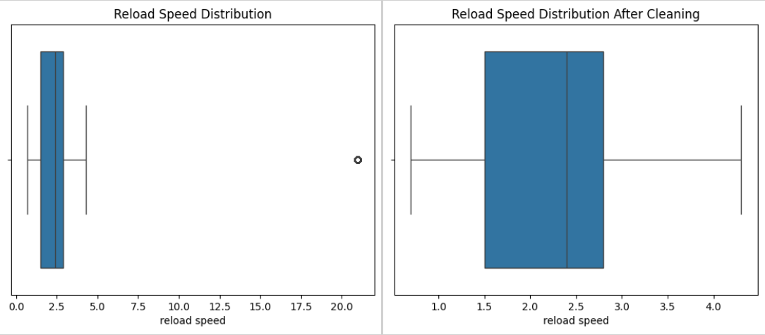
#check for outliers in reload speed
data['reload speed'].unique()
sns.boxplot(data['reload speed'], orient='h')
plt.title('Reload Speed Distribution')
# %%
#drop reload speed outliers
data = data[data['reload speed'] < 10]
sns.boxplot(data['reload speed'], orient='h')
plt.title('Reload Speed Distribution After Cleaning')
# %%
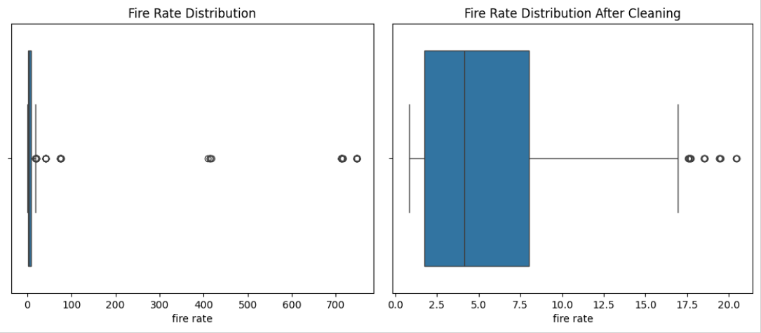
#check for outliers in fire rate
sns.boxplot(data['fire rate'], orient='h')
plt.title('Fire Rate Distribution')
# %%
#drop fire rate outliers
data = data[data['fire rate'] < 40]
sns.boxplot(data['fire rate'], orient='h')
plt.title('Fire Rate Distribution After Cleaning')
# %%
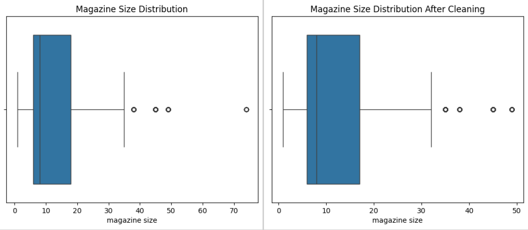
#check for outliers in magazine size
sns.boxplot(data['magazine size'], orient='h')
plt.title('Magazine Size Distribution')
# %%
#drop magazine size outliers
data = data[data['magazine size'] < 70]
sns.boxplot(data['magazine size'], orient='h')
plt.title('Magazine Size Distribution After Cleaning')
# %%
#check for outliers in item score
sns.boxplot(data['item score'], orient='h')
plt.title('Item Score Distribution')
# %%
#drop item score outliers
data = data[data['item score'] < 300]
sns.boxplot(data['item score'], orient='h')
#rename graph
plt.title('Item Score Distribution After Cleaning')
# %%
#change gun name to name and rest of name to suffix
data = data.rename(columns={'gun name': 'name', 'rest of name': 'suffix'})
weapon_type = {
"MANTICORE":"SR",
"NIGHTSHADE": "SMG",
"THORN": "PISTOL",
"PARABLE": "SHOTGUN",
"STOVEPIPE": "SHOTGUN",
"HELICAL": "SR",
"SAGA": "SHOTGUN",
"MAGNOLIA": "SR",
"HOBNAIL": "PISTOL",
"TINTACK": "PISTOL",
"MALLORN": "SR",
"TAMARACK": "SR",
"FOXGLOVE": "SMG",
"KETTLEDRUM": "SHOTGUN",
"BOILERMAKER": "SHOTGUN",
"THUMBSBANE": "PISTOL",
"NETTLE": "SMG",
"RIVETER": "PISTOL",
"WRAITH": "SR",
"EIDOLON": "SR",
"PUSHPIN": "PISTOL",
"BASILISK": "SR",
"RAILSPIKE": "PISTOL",
"BANYAN": "SR",
"BARB": "PISTOL",
"PINION": "SR",
"KOBOLD": "SMG",
"FAE": "SMG",
"HEMLOCK": "SMG",
"MYTHOPEIA": "SHOTGUN",
"SPRIGGAN": "SMG",
"GREENSPINE": "PISTOL",
"RATCHET": "SR"
}
data['type'] = data['name'].apply(lambda x: weapon_type[x])
#final length of data
len(data)
# %%
data.head()
# %%
#export to csv
data.to_csv('weapon_data_processed2.csv', index=False)
# %%
Key Design Features:
- Visuals To Aid In Data Validation: Allowed for collection of data without intrusive methods on the game
- Conversion and Handling of invalid data: Converted the screenshots into numerical data so I could perform analysis on it
- Re-Evaluation of Data and Exporting: Sturctured and Exported the extracted data in a csv format to enhance future readabiliy and usability
Stat Distributions Before and After Processing
Machine Learning Analysis
Developed a weapon playstyle classification model using K-Means clustering and Random Forests to categorize weapons based on performance metrics. This model aids as a way for players to quickly analyze if a new weapon is likely to fit their playstyle, enhancing player experience.
# %%
import pandas as pd
import numpy as np
import matplotlib.pyplot as plt
from sklearn.ensemble import RandomForestClassifier
from sklearn.model_selection import KFold, cross_val_score
from sklearn.decomposition import PCA
from sklearn.model_selection import train_test_split
from scipy.optimize import curve_fit
from sklearn.metrics import accuracy_score, classification_report
from sklearn.cluster import KMeans
from sklearn.preprocessing import LabelEncoder
from sklearn.model_selection import GridSearchCV, ParameterGrid
from sklearn.metrics import confusion_matrix, ConfusionMatrixDisplay
import seaborn as sns
from sklearn.model_selection import KFold
# %%
# Cleaning the data
def clean_df(df):
# drop the rows where the ID column is NaN
df.set_index('ID', inplace=True)
df['Prefix'] = df['Prefix'].fillna('None')
df['Suffix'] = df['Suffix'].fillna('None')
df['Rarity'] = df['Rarity'].replace({'White': 1, 'Green': 2, 'Blue': 3, 'Purple': 4})
df['Element'] = df['Element'].replace({'Physical': 0, 'Ignite': 1, 'Freeze': 1, 'Poison': 1,
'Electrocute': 2, 'Leech': 1})
return df
# %%
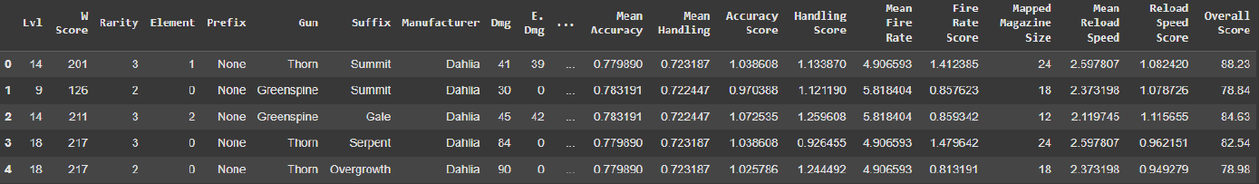
# Loading in the dahlia pistol dataset with the adjusted score metric
dahlia_pistols_df = pd.read_csv('Dahlia_Pistols_Stats.csv')
# Drop the buggy data (Unamed columns)
# dahlia_pistols_df = dahlia_pistols_df.drop(columns=['Unnamed: 30','Unnamed: 31'])
# Cleaning the datafram
dahlia_pistols_df = clean_df(dahlia_pistols_df)
# Checking the rows
dahlia_pistols_df
# %%
# Checking transposed df. Columns Specifically
#dahlia_pistols_df.head().T
# %%
# Create the X train and Y train data
X_train = dahlia_pistols_df.drop(columns=['W Score', 'Prefix', 'Gun', 'Suffix', 'Manufacturer',
'Dmg', 'E. Dmg', 'Chance', 'Elem Bonus', 'Total', 'Value', 'Crit Bonus', 'Acc Eff.', 'Hand Eff.',
'Adj. Eff.', 'Reload Eff.', 'Rate Eff.', 'Total Eff.', 'Total Score', 'Adjusted Score'])
Y_train = dahlia_pistols_df['Gun']
# %%
# Encoded alphabetically Barb:0, Greenspine:1, Thorn:2
label_encoder = LabelEncoder()
# %%
Y_train = label_encoder.fit_transform(Y_train)
# %%
# Importing the test data for the pistols with no parts
dahlia_pistols_np_df = pd.read_csv('Dahlia_Pistols_NP.csv', delimiter= ',')
dahlia_pistols_np_df = clean_df(dahlia_pistols_np_df)
#dahlia_pistols_np_df.head()
# %%
#dahlia_pistols_np_df.head().T
# %%
# Creating the test data. Make X and Y train be only when the level is 3
X_test = dahlia_pistols_np_df.drop(columns=['W Score', 'Prefix', 'Gun', 'Suffix', 'Manufacturer',
'Dmg', 'E. Dmg', 'Chance', 'Elem Bonus', 'Total', 'Value', 'Crit Bonus', 'Acc Eff.', 'Hand Eff.',
'Adj. Eff.', 'Reload Eff.', 'Rate Eff.', 'Total Eff.', 'Total Score', 'Adjusted Score'])
Y_test = dahlia_pistols_np_df['Gun']
# %%
# Encode the test data for prediction. Barb:0, Greenspine:1, Thorn:2
Y_test = label_encoder.fit_transform(Y_test)
y_test_decoded = label_encoder.inverse_transform(Y_test)
# %%
# Creating the forest classifier
w_clf = RandomForestClassifier(random_state=42)
# Parameter grid for optimization
param_grid = {
'n_estimators': [9, 10, 15, 20], # Number of trees
'max_depth': [None, 9, 10], # Maximum depth of each tree
'min_samples_split': [2, 4, 7, 10], # Minimum samples to split a node
'min_samples_leaf': [1, 2], # Minimum samples per leaf
'max_features': ['sqrt', None], # Features considered at each split
}
w_grid_search = GridSearchCV(
estimator=w_clf,
param_grid=param_grid,
cv=8, # 5-fold cross-validation
scoring='f1_macro', # Optimize for f1 macro
n_jobs=-1, # Use all processors
verbose=2 # Verbose output
)
w_grid_search.fit(X_train, Y_train)
# Best parameters and score
print("Best Parameters:", w_grid_search.best_params_)
print("Best Cross-Validation F1 macro:", w_grid_search.best_score_)
# Evaluate the model on the test set
best_rf = w_grid_search.best_estimator_
y_pred = best_rf.predict(X_test)
print(classification_report(Y_test, y_pred))
# %%
kf = KFold(n_splits=8, shuffle=True, random_state=42) #, random_state=42
w_clf = RandomForestClassifier(max_depth = 10, max_features = 'sqrt', n_estimators = 20,
min_samples_leaf = 1, random_state=42, min_samples_split = 2)
w_clf.fit(X_train, Y_train)
Y_pred = w_clf.predict(X_test)
Y_pred_decoded = label_encoder.inverse_transform(Y_pred)
print("Accuracy:", accuracy_score(Y_test, Y_pred))
print("Classification Report:\n", classification_report(Y_test, Y_pred, target_names=label_encoder.classes_))
feature_importances = pd.DataFrame({
'Feature': X_train.columns,
'Importance': w_clf.feature_importances_
}).sort_values(by='Importance', ascending=False)
print("Feature Importances:\n", feature_importances)
scores = cross_val_score(w_clf, X_train, Y_train, cv=kf, scoring='f1_macro')
print(f"Cross-validation accuracy scores: {scores}")
print(f"Mean accuracy: {np.mean(scores):.2f}")
print(f"Standard deviation: {np.std(scores):.2f}")
# %%
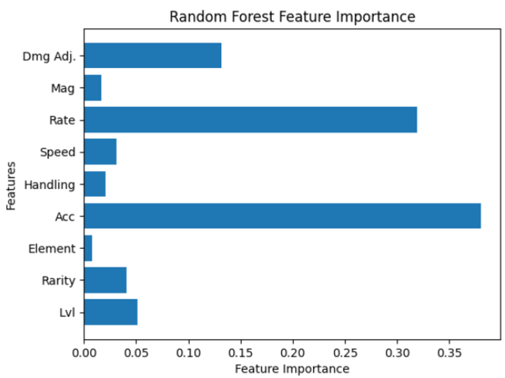
p_importances = w_clf.feature_importances_
w_grid_searchfeature_names = X_train.columns
plt.barh(w_grid_searchfeature_names, p_importances)
plt.xlabel("Feature Importance")
plt.ylabel("Features")
plt.title("Random Forest Feature Importance")
plt.show()
# %%
# Make a dataframe comparing y_predicted to y_test. Make sure both are decoded
#Set the index to the index(ID) from y_test
y_df = pd.DataFrame({'Predicted': Y_pred_decoded, 'Actual': y_test_decoded}, index=dahlia_pistols_np_df.index)
y_df
# %%
# Adjusted the Damage Adjusted Formula by Level
# Setting new variables for the different gun graphs
# Barbs
barb_x_data = dahlia_pistols_df.where(dahlia_pistols_df['Gun'] == 'Barb').dropna()['Lvl']
barb_y_data = dahlia_pistols_df.where(dahlia_pistols_df['Gun'] == 'Barb').dropna()['Dmg Adj.']
# Define the exponential function
def exponential(x, a, b):
return a * np.exp(b * x)
# Fit the data to the exponential model
barb_params, barb_covariance = curve_fit(exponential, barb_x_data, barb_y_data)
barb_a_fit, barb_b_fit = barb_params
# Generate fitted values
barb_y_fit = exponential(barb_x_data, barb_a_fit, barb_b_fit)
# Create a DataFrame for seaborn
barb_plot_df = pd.DataFrame({'Level': barb_x_data, 'Adjusted Damage': barb_y_data})
# Create the plot using seaborn
sns.set_theme(style="darkgrid") # Optional: set a theme
plt.figure(figsize=(10, 6))
sns.regplot(x='Level', y='Adjusted Damage', data=barb_plot_df, order=2,
scatter_kws={'color': 'blue', 's': 50}, line_kws={'color': 'red'}) # order=2 makes the trendline exponential
# Adding details to the graph
plt.title('Barbs: Level vs Adjusted Damage (Exponential Trendline)')
plt.xlabel('Level')
plt.ylabel('Adjusted Damage')
#show the trendline equation
plt.text(0.5, 0.95, f'y = {barb_a_fit:.2f} * e^({barb_b_fit:.2f}x)',
transform=plt.gca().transAxes, fontsize=12, verticalalignment='top')
# show the residuals
plt.scatter(barb_x_data, barb_y_data - barb_y_fit, color='green', label='Residuals')
plt.legend(['Original Data', 'Exponential Trendline'])
plt.grid(True)
plt.show()
print(barb_y_fit)
# %%
# Greenspines
greenspine_x_data = dahlia_pistols_df.where(dahlia_pistols_df['Gun'] == 'Greenspine').dropna()['Lvl']
greenspine_y_data = dahlia_pistols_df.where(dahlia_pistols_df['Gun'] == 'Greenspine').dropna()['Dmg Adj.']
# Fit the data to the exponential model
greenspine_params, greenspine_covariance = curve_fit(exponential, greenspine_x_data, greenspine_y_data)
greenspine_a_fit, greenspine_b_fit = greenspine_params
# Generate fitted values
greenspine_y_fit = exponential(greenspine_x_data, greenspine_a_fit, greenspine_b_fit)
# Create a DataFrame for seaborn
greenspine_plot_df = pd.DataFrame({'Level': greenspine_x_data, 'Adjusted Damage': greenspine_y_data})
# Create the plot using seaborn
sns.set_theme(style="darkgrid") # Optional: set a theme
plt.figure(figsize=(10, 6))
sns.regplot(x='Level', y='Adjusted Damage', data=greenspine_plot_df, order=2,
scatter_kws={'color': 'blue', 's': 50}, line_kws={'color': 'red'}) # order=2 makes the trendline exponential
# Adding details to the graph
plt.title('Greeenspine: Level vs Adjusted Damage (Exponential Trendline)')
plt.xlabel('Level')
plt.ylabel('Adjusted Damage')
#show the trendline equation
plt.text(0.5, 0.95, f'y = {greenspine_a_fit:.2f} * e^({greenspine_b_fit:.2f}x)',
transform=plt.gca().transAxes, fontsize=12, verticalalignment='top')
# show the residuals
plt.scatter(greenspine_x_data, greenspine_y_data - greenspine_y_fit, color='green', label='Residuals')
plt.legend(['Original Data', 'Exponential Trendline'])
plt.grid(True)
plt.show()
print(greenspine_y_fit)
# %%
# Thorns
thorn_x_data = dahlia_pistols_df.where(dahlia_pistols_df['Gun'] == 'Thorn').dropna()['Lvl']
thorn_y_data = dahlia_pistols_df.where(dahlia_pistols_df['Gun'] == 'Thorn').dropna()['Dmg Adj.']
# Fit the data to the exponential model
thorn_params, thorn_covariance = curve_fit(exponential, thorn_x_data, thorn_y_data)
thorn_a_fit, thorn_b_fit = thorn_params
# Generate fitted values
thorn_y_fit = exponential(thorn_x_data, thorn_a_fit, thorn_b_fit)
# Create a DataFrame for seaborn
thorn_plot_df = pd.DataFrame({'Level': thorn_x_data, 'Adjusted Damage': thorn_y_data})
# Create the plot using seaborn
sns.set_theme(style="darkgrid") # Optional: set a theme
plt.figure(figsize=(10, 6))
sns.regplot(x='Level', y='Adjusted Damage', data=thorn_plot_df, order=2,
scatter_kws={'color': 'blue', 's': 50}, line_kws={'color': 'red'}) # order=2 makes the trendline exponential
# Adding details to the graph
plt.title('Thorns: Level vs Adjusted Damage (Exponential Trendline)')
plt.xlabel('Level')
plt.ylabel('Adjusted Damage')
# Show the trendline equation
plt.text(0.5, 0.95, f'y = {thorn_a_fit:.2f} * e^({thorn_b_fit:.2f}x)',
transform=plt.gca().transAxes, fontsize=12, verticalalignment='top')
# Show the residuals
plt.scatter(thorn_x_data, thorn_y_data - thorn_y_fit, color='green', label='Residuals')
plt.legend(['Original Data', 'Exponential Trendline'])
plt.grid(True)
plt.show()
print(thorn_y_fit)
# %%
# Define the exponential function for damage calculation
def log_calculate_damage(level):
return 13 * (np.log(level + 2))
# Maximum level (assumed to be 40 for this example)
max_level = 40
# Calculate the maximum damage at level 40 for normalization
max_damage = 600
# %%
# Function to calculate and normalize damage for each gun
def normalize_damage(level):
base_damage = log_calculate_damage(level)
normalized_damage = base_damage / max_damage
return normalized_damage
log_normalized_damage_values = [normalize_damage(level) for level in range(1, max_level + 1)]
# Output normalized damage values for reference
# print(log_normalized_damage_values)
# Apply the normalization function to the 'Level' column in the dataset
dahlia_pistols_df['Normalized Damage By Lvl'] = (dahlia_pistols_df['Lvl'].apply(normalize_damage)) * 10
dahlia_pistols_df['Normalized Damage Adjusted'] = dahlia_pistols_df['Dmg Adj.'].apply(normalize_damage) * 10
dahlia_pistols_df['New Damage Adjusted'] = dahlia_pistols_df['Normalized Damage Adjusted']
/ dahlia_pistols_df['Normalized Damage By Lvl']
# Display the updated dataset with normalized damage values
# dahlia_pistols_df.head(20)
# %%
new_cleaned_up_table = dahlia_pistols_df.drop(columns = ['Dmg Adj.', 'Acc Eff.', 'Hand Eff.',
'Adj. Eff.', 'Reload Eff.', 'Rate Eff.', 'Total Eff.', 'Total Score', 'Adjusted Score'])
new_cleaned_up_table['Accuracy Efficiency'] = (new_cleaned_up_table['Acc'] / 100)
new_cleaned_up_table['Handling Efficiency'] = (new_cleaned_up_table['Handling'] / 100)
# %%
# Find the mean accuracy for each gun type
mean_accuracy = new_cleaned_up_table.groupby('Gun')['Accuracy Efficiency'].mean()
# Rename column to Average Accuracy
mean_accuracy = mean_accuracy.rename('Mean Accuracy')
# %%
# Find the mean handling for each gun type
mean_handling = new_cleaned_up_table.groupby('Gun')['Handling Efficiency'].mean()
# Rename column to Average Handling
mean_handling = mean_handling.rename('Mean Handling')
# %%
# Making an Accuracy Score/ Handling Score for different gun types and compiling it into one column
# Make sure it refers to the mean accuracy/handling dataframes when comparing the accuracy/handling.
# Make it so the Score is gun dependent
# Make sure to standardize these numbers so they are between 0 and 1.
new_cleaned_up_table = new_cleaned_up_table.merge(mean_accuracy, on='Gun')
new_cleaned_up_table = new_cleaned_up_table.merge(mean_handling, on='Gun')
# %%
new_cleaned_up_table['Accuracy Score'] = new_cleaned_up_table['Accuracy Efficiency']
/ new_cleaned_up_table['Mean Accuracy']
new_cleaned_up_table['Handling Score'] = new_cleaned_up_table['Handling Efficiency']
/ new_cleaned_up_table['Mean Handling']
# %%
# Start creating the rate efficiency metric by doing the same processes for accuracy and handling
mean_fire_rate = new_cleaned_up_table.groupby('Gun')['Rate'].mean()
mean_fire_rate = mean_fire_rate.rename('Mean Fire Rate')
# %%
new_cleaned_up_table = new_cleaned_up_table.merge(mean_fire_rate, on='Gun')
# %%
new_cleaned_up_table['Fire Rate Score'] = new_cleaned_up_table['Rate'] / new_cleaned_up_table['Mean Fire Rate']
# %%
# Recreate the reload speed efficiency metric
reload_speed_eff = new_cleaned_up_table.groupby('Mag')['Speed'].mean()
reload_speed_eff = reload_speed_eff.rename('Mean Reload Speed')
# %%
# Example mapping dictionary
magazine_size_mapping = {
12: 12, 14: 12, # Group 12 and 14 together
18: 18, 21: 18, # Group 18 and 21 together
24: 24, 29: 24 # Group 24 and 29 together
}
# Recreate the reload speed efficiency metric
reload_speed_eff = reload_speed_eff.to_frame()
reload_speed_eff = reload_speed_eff.reset_index()
reload_speed_eff['Mapped Magazine Size'] = reload_speed_eff['Mag'].map(magazine_size_mapping)
reload_speed_eff = reload_speed_eff.groupby('Mapped Magazine Size')['Mean Reload Speed'].mean()
reload_speed_eff = reload_speed_eff.reset_index()
# %%
new_cleaned_up_table['Mapped Magazine Size'] = new_cleaned_up_table['Mag'].map(magazine_size_mapping)
new_cleaned_up_table = new_cleaned_up_table.merge(reload_speed_eff, on='Mapped Magazine Size')
# %%
new_cleaned_up_table['Reload Speed Score'] = new_cleaned_up_table['Mean Reload Speed'] / new_cleaned_up_table['Speed']
# %%
Overall_Acc = new_cleaned_up_table['Accuracy Score'] / new_cleaned_up_table['Accuracy Score'].max()
Overall_Hand = new_cleaned_up_table['Handling Score'] / new_cleaned_up_table['Handling Score'].max()
Overall_Fire = new_cleaned_up_table['Fire Rate Score'] / new_cleaned_up_table['Fire Rate Score'].max()
Overall_Reload = new_cleaned_up_table['Reload Speed Score'] / new_cleaned_up_table['Reload Speed Score'].max()
overall = np.array([Overall_Acc, Overall_Hand, Overall_Fire, Overall_Reload])
new_cleaned_up_table['Overall Score'] = np.round((np.mean(overall, axis=0) * 100), 2)
new_cleaned_up_table.head()
# %%
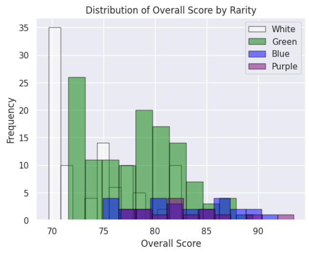
from matplotlib import pyplot as plt
rarities = [1, 2, 3, 4]
colors = ['white', 'green', 'blue', 'purple']
# Seaborn overlayed histogram for the new_cleaned_up_table
sns.set_theme(style="darkgrid")
# Plot a histogram for each rarity
for rarity, color in zip(rarities, colors):
subset = new_cleaned_up_table[new_cleaned_up_table['Rarity'] == rarity]
plt.hist(
subset['Overall Score'],
bins=11, # Adjust the number of bins as needed
alpha=0.5, # Transparency for overlay
label=subset['Rarity'],
color=color,
edgecolor='black'
)
# Make it so that in the legend 1 is changed to white 2 to green 3 to blue and 4 to purple
plt.legend(['White', 'Green', 'Blue', 'Purple'])
plt.xlabel('Overall Score')
plt.ylabel('Frequency')
plt.title('Distribution of Overall Score by Rarity')
plt.show()
# %%
# Plot a graph that will best show the difference between an weapon's item score and our new total score
# Option 1: Scatter Plot with Line of Equality
# Color the dots with the rarity
plt.figure(figsize=(8, 6))
sns.scatterplot(data=new_cleaned_up_table, x='W Score', y='Overall Score', alpha=0.7,
hue = 'Rarity', palette = ['Gray', 'Green', 'Blue', 'Purple'])
plt.xlabel('Item Score')
plt.ylabel('Overall Score')
plt.title('Item Score vs. New Overall Score')
plt.legend(title='Rarity', loc='upper left')
plt.show()
# %%
# Loading in the new bigger dataset
all_weapons_df = pd.read_csv('weapon_data_processed.csv')
all_weapons_df
# %%
# Function to split and multiply the values
# Cleaning the data
def improved_clean_df(df):
# drop the rows where the ID column is NaN
df.rename(columns = {'rarity' : 'Rarity'}, inplace=True)
df['Rarity'] = df['Rarity'].replace({'COMMON': 1, 'UNCOMMON': 2, 'RARE': 3, 'EPIC': 4})
# Renaming
df.rename(columns = {'damage' : 'Damage'}, inplace=True)
# Rename the accuracy column
df.rename(columns = {'accuracy' : 'Accuracy'}, inplace=True)
# Rename the handling column
df.rename(columns = {'handling' : 'Handling'}, inplace=True)
# Rename the rate column
df.rename(columns = {'fire rate' : 'Fire Rate'}, inplace=True)
# Rename the reload speed column
df.rename(columns = {'reload speed' : 'Reload Speed'}, inplace=True)
# Rename the magazine column
df.rename(columns = {'magazine size' : 'Magazine'}, inplace=True)
#df['elemental damage'] = df['elemental damage'].str.replace(r'^[.,](?=\d)', '', regex=True)
#df['elemental chance'] = df['elemental chance'].str.replace(r'^[.,](?=\d)', '', regex=True)
# Rename them
df.rename(columns = {'elemental damage' : 'Elemental Damage'}, inplace=True)
df.rename(columns = {'elemental chance' : 'Elemental Chance'}, inplace=True)
# df['Element'] = df['Element'].replace({'Physical': 0, 'Ignite': 1, 'Freeze': 1,
'Poison': 1, 'Electrocute': 2, 'Leech': 1})
# Rename the name column
df.rename(columns = {'name' : 'Name'}, inplace=True)
# Gun type is the first word of name
df['Gun Type'] = df['Name'].apply(lambda x: x.split()[0])
# Rename the item score column
df.rename(columns = {'item score' : 'Item Score'}, inplace=True)
# Fix the damage column so that values like 6x6 are changed to 36 as in the x indicates multiplication
# Then make the damage the result of multiplying the 2 said numbers
# Apply the mulplier
df['Damage'] = df['Damage'].astype(int)
df['Elemental Chance'] = pd.to_numeric(df['Elemental Chance'])
df['Elemental Damage'] = pd.to_numeric(df['Elemental Damage'])
return df
all_weapons_df = improved_clean_df(all_weapons_df)
all_weapons_df
# %%
# Find the unique manufacturers from the manufacturer column
unique_manufacturers = all_weapons_df['manufacturer'].unique()
unique_gun_types = all_weapons_df['Gun Type'].unique()
unique_gun_types
# %%
# Create the train and test set from the all weapon df
features = all_weapons_df.drop(columns=['Item Score', 'Gun Type', 'Name',
'suffix', 'manufacturer']) # Drop the target column
target = all_weapons_df['Gun Type']
target_encoded = label_encoder.fit_transform(target)
all_X_train, all_X_test, all_y_train, all_y_test = train_test_split(features, target_encoded,
test_size=0.2, random_state = 42)
all_weapons_clf = RandomForestClassifier(max_depth = None, max_features = 'sqrt',
n_estimators = 100, min_samples_leaf = 1, random_state=42, min_samples_split = 2)
all_weapons_clf.fit(all_X_train, all_y_train)
all_y_pred = all_weapons_clf.predict(all_X_test)
all_y_pred_decoded = label_encoder.inverse_transform(all_y_pred)
all_y_test_decoded = label_encoder.inverse_transform(all_y_test)
# %%
print("Accuracy:", accuracy_score(all_y_test, all_y_pred))
unique_classes = np.unique(np.concatenate((all_y_test, all_y_pred)))
target_names = label_encoder.inverse_transform(unique_classes)
print("Classification Report:\n", classification_report(all_y_test, all_y_pred, target_names=target_names))
# Step 7: Feature Importance (Optional)
feature_importances = pd.DataFrame({
'Feature': features.columns,
'Importance': all_weapons_clf.feature_importances_
}).sort_values(by='Importance', ascending=False)
print("Feature Importances:\n", feature_importances)
# %%
# Make a dataframe comparing all_y_predicted to all_y_test. Make sure both are decoded
#all_y_df = pd.DataFrame({'Predicted': all_y_pred_decoded, 'Actual': all_y_test_decoded},
index=dahlia_pistols_np_df.index)
all_y_df = pd.DataFrame({'Predicted': all_y_pred_decoded, 'Actual': all_y_test_decoded})
all_y_df
# %%
# table display of incorrect counts
all_y_df_c = all_y_df.copy()
all_y_df_c['Correct'] = (all_y_df_c['Predicted'] == all_y_df_c['Actual']).astype(int)
incorrect_pred = all_y_df_c[all_y_df_c['Correct'] == 0]
incorrect_pred = incorrect_pred.groupby(['Predicted', 'Actual']).count()
incorrect_pred = incorrect_pred.rename(columns={'Correct': 'Count'})
incorrect_pred = incorrect_pred.sort_values(by='Count', ascending=False)
incorrect_pred
# %%
# making a confusion matrix for misclassified counts heatmap
cm = confusion_matrix(all_y_test, all_y_pred)
misclassified_matrix = cm.copy()
np.fill_diagonal(misclassified_matrix, 0)
plt.figure(figsize=(10, 8))
sns.heatmap(misclassified_matrix, annot=True, fmt="d", cmap="Reds",
xticklabels= label_encoder.classes_,
yticklabels= label_encoder.classes_)
plt.title("Misclassified Counts Heatmap")
plt.xlabel("Predicted Class")
plt.ylabel("True Class")
plt.show()
# %%
playstyledf = pd.read_csv('weapon_data_processed10.csv')
playstyledf['rarity'] = playstyledf['rarity'].replace({'COMMON': 1, 'UNCOMMON': 2, 'RARE': 3, 'EPIC': 4})
playstyledf.head()
# %%
from sklearn.preprocessing import StandardScaler
playstyledf['suffix'] = playstyledf['suffix'].fillna('NONE')
numeric_columns = ['damage', 'fire rate', 'accuracy', 'handling', 'reload speed','magazine size']
features = playstyledf[numeric_columns]
scaler = StandardScaler()
features_scaled = scaler.fit_transform(features)
playstyledf.head()
# %%
features_scaled = pd.DataFrame(features_scaled, columns=numeric_columns)
features_scaled.head()
# %%
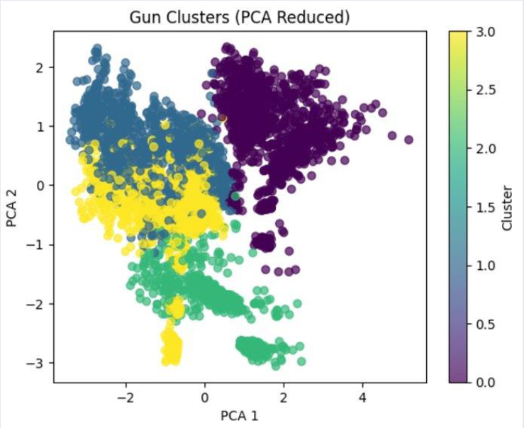
#k-means clustering to cluster weapons into playstyles
n_clusters = 4
kmeans = KMeans(n_clusters=n_clusters, random_state=42)
playstyledf['Cluster'] = kmeans.fit_predict(features_scaled)
#cluster visuals
pca = PCA(n_components=2)
pca_features = pca.fit_transform(features_scaled)
plt.scatter(pca_features[:, 0], pca_features[:, 1], c=playstyledf['Cluster'], cmap='viridis', alpha=0.7)
plt.title('Gun Clusters (PCA Reduced)')
plt.xlabel('PCA 1')
plt.ylabel('PCA 2')
plt.colorbar(label='Cluster')
plt.show()
# %%
#check which guns are in each cluster
for i in range(n_clusters):
print(f'Cluster {i}:')
print(playstyledf[playstyledf['Cluster'] == i]['name'].values)
# whats the most common type for each cluster
for i in range(n_clusters):
print(f'Cluster {i}:')
print(playstyledf[playstyledf['Cluster'] == i]['type'].value_counts().idxmax())
# %%
#what percentage of each cluster is each type
for i in range(n_clusters):
print(f'Cluster {i}:')
print(playstyledf[playstyledf['Cluster'] == i]['type'].value_counts(normalize=True))
# %%
#add the cluster column to the dataframe
playstyledf['Cluster'] = playstyledf['Cluster'].astype(str)
playstyledf.head()
# %%
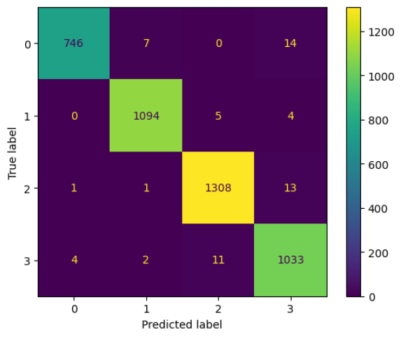
#build a model to predict the cluster
X = features_scaled
y = playstyledf['Cluster']
X_train, X_test, y_train, y_test = train_test_split(X, y, test_size=0.2, random_state=42)
# Random Forest
rf = RandomForestClassifier(random_state=42)
rf.fit(X_train, y_train)
y_pred = rf.predict(X_test)
print(f'Accuracy: {accuracy_score(y_test, y_pred)}')
print(classification_report(y_test, y_pred))
# %%Model Features:
- Data Analysis of Weapon Metrics: Goals, assists, minutes played, ratings
- Derived New Metric: Overall score based on combination of stats
- K-Means Clustering: Used a combination of PCA and K-Means to cluster weapons into 4 playstyles
- Test and Training split: Split my data into test and train sets to validate model performance
Model Visualizations
Results & Impact
Data Creation
Created a dataset that wouldn't normally be obtainable by using automated OCR to extract data directly from the game
Model Accuracy
The model was able to predict which cluster a never before seen weapon would fall into with 98% accuracy
Stakeholder Presentation
Created and presented a slideshow explaining the entire project so non-technical stakeholders would be able to understand